Utopia, you are standing in it!

Most Keynesian economists are convinced that something exists called involuntary unemployment and people can be unemployed through no fault of their own. They will accept the going wage but no employer is willing to offer it to them.

Lucas and Rapping’s (1969) paper, “Real Wages, Employment, and Inflation” provides the micro-foundations for an analysis of the labour suppl. They felt the need to reconcile the existence of unemployment with market clearing and referred to recent work of Armen Alchian (1969) on search explanations of unemployment.

Lucas and Rapping viewed unemployment as voluntary, including the mass unemployment during the great depression (Lucas and Rapping 1969: 748).

Lucas and-Rapping viewed current labour demand as a negative function of the current real wage. Current labour supply was a positive function of the real wage and the expected real interest rate, but a negative function of the expected future wage.

Under their framework, if workers expect higher real wages in the future or a lower real interest rate, current labour supply would be depressed, employment would fall, unemployment rise, and real wages increase.

Lucas and Rapping depicted labour suppliers as rational optimisers who engaged in inter-temporal substitution: working more when current wages were high relative to expected wages. The prevailing Keynesian approach assumed labour supply was passive, and movements in the demand for labour determined changes in employment.

Lucas and Rapping offered an unemployment equation relating the unemployment rate to actual versus anticipated nominal wages, and actual versus anticipated price levels. Unemployment could be the product of expectational errors about wages.

Lucas and Rapping’s model was poor at explaining unemployment after 1933 in terms of job search and expectational errors.

The graph below shows two different series for unemployment in the 1930s in the USA: the official BLS level by Lebergott; and a data series constructed famously by Darby. Darby includes workers in the emergency government labour force as employed – the most important being the Civil Works Administration (CWA) and the Works Progress Administration (WPA).

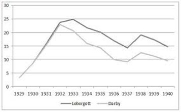
Once these workfare programs are accounted for, the level of U.S. unemployment fell from 22.9% in 1932 to 9.1% in 1937, a reduction of 13.8%. For 1934-1941, the corrected unemployment levels are reduced by two to three-and-a half million people and the unemployment rates by 4 to 7 percentage points after 1933.

Not surprisingly, Darby titled his 1976 Journal of Political Economy article Three-and-a-Half Million U.S. Employees Have Been Mislaid: Or, an Explanation of Unemployment, 1934-1941.

The corrected data by Darby shows stronger movement toward the natural unemployment rate after 1933. Darby concluded that his corrected date are suggests that the unemployment rate was well explained by a job search model such as that by Lucas and Rapping together with the wage fixing under the New Deal that kept real wages up and unemployment high.

Both the Keynesian approach to unemployment and the job search approach to unemployment view workers in emergency government work programs as employed and not as unemployed.

In the late 1970s, Modigliani dismissed the new classical explanation of the U.S. great depression in which the 1930s unemployment was mass voluntary unemployment as follows:

Sargent (1976) has attempted to remedy this fatal flaw by hypothesizing that the persistent and large fluctuations in unemployment reflect merely corresponding swings in the natural rate itself.

In other words, what happened to the U.S. in the 1930’s was a severe attack of contagious laziness!

I can only say that, despite Sargent’s ingenuity, neither I nor, I expect most others at least of the nonMonetarist persuasion,. are quite ready yet. to turn over the field of economic fluctuations to the social psychologist!

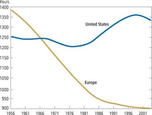
As Prescott has pointed out, the USA in the Great Depression and France since the 1970s both had 30% drops in hours worked per adult. That is why Prescott refers to France’s economy as depressed. The reason for the depressed state of the French (and German) economies is taxes, according to Prescott:

Virtually all of the large differences between U.S. labour supply and those of Germany and France are due to differences in tax systems.

Europeans face higher tax rates than Americans, and European tax rates have risen significantly over the past several decades.

In the 1960s, the number of hours worked was about the same. Since then, the number of hours has stayed level in the United States, while it has declined substantially in Europe. Countries with high tax rates devote less time to market work, but more time to home activities, such as cooking and cleaning. The European services sector is much smaller than in the USA.

Time use studies find that lower hours of market work in Europe is entirely offset by higher hours of home production, implying that Europeans do not enjoy more leisure than Americans despite the widespread impression that they do.

Richard Rogerson, 2007 in “Taxation and market work: is Scandinavia an outlier?” found that how the government spends tax revenues when assessing the effects of tax rates on aggregate hours of market work:

1. Different forms of government spending imply different elasticities of hours of work with regard to tax rates;
2. While tax rates are highest in Scandinavia, hours worked in Scandinavia are significantly higher than they are in Continental Europe with differences in the form of government spending can potentially account for this pattern; and
3. There is a much higher rate of government employment and greater expenditures on child and elderly care in Scandinavia.

Examining how tax revenue is spent is central to understanding labour supply effects:

1. If higher taxes fund disability payments which may only be received when not in work, the effect on hours worked is greater relative to a lump-sum transfer; and
2. If higher taxes subsidise day care for individuals who work, then the effect on hours of work will be less than under the lump-sum transfer case.

Others such as Blanchard attribute the much lower labour force participation in the EU since the 1970s to their greater preference for leisure in Europe. An increased preference for leisure is another name for voluntary unemployment.

The lower labour force participation in higher unemployment in Europe is voluntary because of the higher demand for leisure among Europeans.  According to Blanchard:

The main difference [between the continents] is that Europe has used some of the increase in productivity to increase leisure rather than income, while the U.S. has done the opposite.

An unusual left-right unity ticket emerged to explain the great depression in the 1930s and the depressed EU economies from the 1970s: the great vacation theory.