Economists, using charts or high-speed computer models, can accurately forecast the future
01 Jul 2014 Leave a comment
in entrepreneurship, macroeconomics, Murray Rothbard Tags: forecasting errors, Murray Rothbard, The pretence to knowledge

Many studies, formal and informal, have been made of the record of forecasting by economists, and it has been consistently abysmal.
Forecasters often complain that they can do well enough as long as current trends continue; what they have difficulty in doing is catching changes in trend. But of course there is no trick in extrapolating current trends into the near future.
You don’t need sophisticated computer models for that; you can do it better and far more cheaply by using a ruler.
The real trick is precisely to forecast when and how trends will change, and forecasters have been notoriously bad at that. No economist forecast the depth of the 1981–82 depression, and none predicted the strength of the 1983 boom.
The next time you are swayed by the jargon or seeming expertise of the economic forecaster, ask yourself this question: If he can really predict the future so well, why is he wasting his time putting out newsletters or doing consulting when he himself could be making trillions of dollars in the stock and commodity markets?

Milton Friedman on what presidents can do to increase the economic growth rate
28 Jun 2014 1 Comment
in economic growth, macroeconomics, Milton Friedman Tags: Milton Friedmand, The fatel conceit, The pretense to knowledge
First of all, I don’t think the president has a great deal to do with keeping the economy going…
I think presidents have a great deal to do with keeping the economy from growing…
I think the economy is largely independent of the government, and what keeps it going is its own internal development.
However, you can short-circuit that internal development. If you impose very high taxes, and eliminate the incentive to innovate, to improve, to take risks, and do things, you’ll kill the economy. And that’s what’s happened over and over again in other countries around the world.
Is unemployment voluntary or involuntary?
27 Jun 2014 Leave a comment
in business cycles, job search and matching, labour economics, macroeconomics, unemployment Tags: Alan Manning, Armen Alchian, Robert Barro, Robert Lucas, unemployment

Robert Lucas in a famous 1978 paper argued that all unemployment was voluntary because involuntary unemployment was a meaningless concept. He said as follows:
The worker who loses a good job in prosperous time does not volunteer to be in this situation: he has suffered a capital loss. Similarly, the firm which loses an experienced employee in depressed times suffers an undesirable capital loss.
Nevertheless the unemployed worker at any time can always find some job at once, and a firm can always fill a vacancy instantaneously. That neither typically does so by choice is not difficult to understand given the quality of the jobs and the employees which are easiest to find.
Thus there is an involuntary element in all unemployment, in the sense that no one chooses bad luck over good; there is also a voluntary element in all unemployment, in the sense that however miserable one’s current work options, one can always choose to accept them.
I agree that we all make choices subject to constraints. To say that a choice is involuntary because it is constrained by a scarcity of job-opportunities information is to say that choices are involuntary because there is scarcity.
Alchian said there are always plenty of jobs because to suppose the contrary suggests that scarcity has been abolished. Lucas elaborated further in 1987 in Models of Business Cycles:
A theory that does deal successfully with unemployment needs to address two quite distinct problems.
One is the fact that job separations tend to take the form of unilateral decisions – a worker quits, or is laid off or fired – in which negotiations over wage rates play no explicit role.
The second is that workers who lose jobs, for whatever reason, typically pass through a period of unemployment instead of taking temporary work on the ‘spot’ labour market jobs that are readily available in any economy.
Of these, the second seems to me much the more important: it does not ‘explain’ why someone is unemployed to explain why he does not have a job with company X. After all, most employed people do not have jobs with company X either.
To explain why people allocate time to a particular activity – like unemployment – we need to know why they prefer it to all other available activities: to say that I am allergic to strawberries does not ‘explain’ why I drink coffee. Neither of these puzzles is easy to understand within a Walrasian framework, and it would be good to understand both of them better, but I suggest we begin by focusing on the second of the two.
Another way to understand unemployment is to use a device at the start of Alan Manning’s book on labour market monopsony:
What happens if an employer cuts the wage it pays its workers by one cent? Much of labour economics is built on the assumption that all existing workers immediately leave the firm as that is the implication of the assumption of perfect competition in the labour market.
In such a situation an employer faces a market wage for each type of labour determined by forces beyond its control at which any number of these workers can be hired but any attempt to pay a lower wage will result in the complete inability to hire any of them at all
Suppose workers offered to work for 1 cent. Would employers accept? Many do because they have intern and work experience programmes for students, but is this result of general application?
Understanding the reallocation of labour at the end of the recession requires careful attention to the 1980s writing of Alchian on the theory of the firm. Alchian and Woodward’s 1987 ‘Reflections on a theory of the firm’ says:
… the notion of a quickly equilibrating market price is baffling save in a very few markets. Imagine an employer and an employee. Will they renegotiate price every hour, or with every perceived change in circumstances?
If the employee is a waiter in a restaurant, would the waiter’s wage be renegotiated with every new customer? Would it be renegotiated to zero when no customers are present, and then back to a high level that would extract the entire customer value when a queue appears?
… But what is the right interval for renegotiation or change in price? The usual answer ‘as soon as demand or supply changes’ is uninformative.
Alchian and Woodward then go on to a long discussion of the role of protecting composite quasi-rents from dependent resources as the decider of the timing of wage and price revisions.
Alchian and Woodward explain unemployment as a side-effect of the purpose of wage and price rigidity, which is the prevention of hold-ups over dependent assets. They note that unemployment cannot be understood until an adequate theory of the firm explains the type of contracts the members of a firm make with one another.
My interpretation is the majority of employment relationships are capital intensive long-term contracts. Employers spend a lot of time searching and screening applicants to find those that will stay longer. In less skilled jobs, and in spot market jobs, employers will hire the best applicant quickly because job turnover costs are low. Back to Manning again:
That important frictions exist in the labour market seems undeniable: people go to the pub to celebrate when they get a job rather than greeting the news with the shrug of the shoulders that we might expect if labour markets were frictionless. And people go to the pub to drown their sorrows when they lose their job rather than picking up another one straight away. The importance of frictions has been recognized since at least the work of Stigler (1961, 1962).
Whatever may be among these frictions, wage rigidity is not one of them. Wages are flexible for job stayers and certainly new starters.
See What can wages and employment tell us about the UK’s productivity puzzle? by Richard Blundell, Claire Crawford and Wenchao Jin showing that in the recent UK recession 12% of employees in the same job as 12 months ago experienced wage freezes and 21% of workers in the same job as 12 months ago experienced wage cuts. Their data covered 80% of workers in the New Earnings Survey Panel Dataset.
Larger firms lay off workers; smaller firms tended to reduce wages. This British data showing widespread wage cuts dates back to the 1980s. Recent Irish data also shows extensive wage cuts among job stayers.
See too Chris Pissarides (2009), The Unemployment Volatility Puzzle: Is Wage Stickiness the Answer? arguing the wage stickiness is not the answer since wages in new job matches are highly flexible:
- wages of job changers are always substantially more procyclical than the wages of job stayers.
- the wages of job stayers, and even of those who remain in the same job with the same employer are still mildly procyclical.
- there is more procyclicality in the wages of stayers in Europe than in the United States.
- The procyclicality of job stayers’ wages is sometimes due to bonuses, and overtime pay but it still reflects a rise in the hourly cost of labour to the firm in cyclical peaks
How do existing firms who will not cut wages survive in competition with new firms who can start workers on lower wages? Industries with many short term jobs and seasonal jobs would suffer less from wage inflexibility.
Robert Barro (1977) pointed out that wage rigidity matters little because workers can, for example, agree in advance that they will work harder when there is more work to do—that is, when the demand for a firm’s product is high—and work less hard when there is little work. Stickiness of nominal wage rates does not necessarily cause errors in the determination of labour and production.
The ability to make long-term wage contracts and include clauses that guard against opportunistic wage cuts should make the parties better off. Workers will not sign these contracts if they are against their interests. Employers do not offer these contracts, and offer more flexible wage packages, will undercut employers who are more rigid. Furthermore many workers are on performance pay that link there must wages to the profitability of the company.
How can downward wage rigidity be a scientific hypothesis if extensive international evidence of widespread wage cuts since the 1980s and 30%+ of the workforce on performance bonuses is not enough to refute it?
Alchian and Kessel in “The Meaning and Validity of the Inflation-Induced Lag of Wages Behind Prices,” Amer. Econ. Rev. 50 [March 1960]:43-66) tested the hypothesis that workers suffered from money illusion by comparing the rates of return to firms in capital intensive industries with those of labour intensive industries. Labour intensive industries were not more profitable than capital intensive industries. Employers in labour intensive industries should profit from the misperceptions of workers about wages and future prices, but they did not. Alchian and Kessel found little evidence of a lag between wage and price changes.
In Canadian industries in the 1960s and 1970s, wage indexation ranged from zero to nearly 100%. Industries with little indexation should show substantial responses of real wage rates, employment and output to nominal shocks. Industries with lots of indexation would be affected little by nominal disturbances. Monetary shocks had positive effects but an industry’s response to these shocks bore no relation to the amount of indexation in the industry. Shaghil Ahmed (1987) found that those industries with lots of indexation were as likely as those with little indexation to respond to shocks.
If the signing of new wage contracts was important to wage rigidity, there should be unusual behaviour of employment and real wage rates just after these signings, but the results are mixed. Olivei and Tenreyro (2010) used the tendency of contracts to be signed at the start of years to show that monetary policy had significant effects in January but little effect in December because the effects were quickly undone.
Alchian (1969) lists three ways to adjust to unanticipated demand fluctuations:
• output adjustments;
• wage and price adjustments; and
• Inventories and queues (including reservations).
Alchian (1969) suggests that there is no reason for wage and price changes to be used regardless of the relative cost of these other options:
• The cost of output adjustment stems from the fact that marginal costs rise with output;
• The cost of price adjustment arises because uncertain prices and wages induce costly search by buyers and sellers seeking the best offer; and
• The third method of adjustment has holding and queuing costs.
There is a tendency for unpredicted price and wage changes to induce costly additional search. Long-term contracts including implicit contracts arise to share risks and curb opportunism over relationship-specific capital. These factors lead to queues, unemployment, spare capacity, layoffs, shortages, inventories and non-price rationing in conjunction with wage stability.
Are you now or have you ever been a monetarist?
26 Jun 2014 Leave a comment
in macroeconomics, Milton Friedman, monetarism Tags: Milton Friedman, monetarism, The Fed

Milton Friedman argued that no member of the Fed would have ever answered yes to that question.
The Schumpeterian view of business cycles
26 Jun 2014 Leave a comment
in business cycles, macroeconomics Tags: business cycles, David Andolfatto, Schumpeter

David Andolfatto argues for the Schumpeterian view of economic development where the distinction between growth and business cycles is artificial. Everyone agrees that long-run growth is the product of technological advancement. The Keynesian school views trend growth as being stable with new technologies unfolding at a smooth rate.

In the Schumpeterian view, there is no reason to believe that the process of technological advancement is smooth. It is more reasonable to suppose that new technologies appear in clusters.
There will be incremental innovations, and from time to time, grand innovations that transformed the entire economy. These grand innovations require the economy to slow down while it invests in a whole range of secondary innovations to make the most of these great new technologies. Writing workable software for new computers is an example.
These technology shocks may cause fluctuations in the growth rate through what Schumpeter called a process of creative destruction. Innovations cluster in specific industries and this generates the boom. When the cluster of innovation comes to an end in a particular sector, there is a generally increased risk of failure as old and new firms and entrepreneurs and investors adapt themselves to the new situation.
If business cycles come from innovation, they are an essential feature of economic development. They cannot be eliminated without harming innovation so we should not be too quick to smooth out the business cycle.
Technological advancements that ultimately lead to higher productivity may, in the short run, induce cyclical adjustments as the economy restructures: resources flow out from declining sectors to the expanding sectors, and people retrain and learn the next technologies and invest in the secondary innovations to make, for example, new computers to be of practical application. The first innovators will find the job a difficult one, later innovators will find things very easy, and the last to adopt the innovation will find not much to do. Faster or slower adoption of new technologies will have important implications for production, investment and consumption.

There is no guarantee that all new technologies will work out as planned. What may have looked promising may turn out to be a disappointment.
This leads to the role in news on the business cycle. Obviously, people form expectations about future technologies and invest and consume in the expectation of better or worse times ahead. They will adjust investor and consumer expectations as new information of varying and conflicting quality becomes available about technological prospects and the success of technological developments to date.
Output and employment will go up and down on the basis of these shifting expectations. These shifts in expectations are perfectly rational and are made on the basis of new information about the prospects and performance of new and existing technologies. Of course, some of these forecasts will turn out to be a disappointment and there will be a slowdown in the economy as people regroup.
The problem is not a lack of accurate forecasting by both the old and new firms. If technologies come in clusters, and are clustered in industries, there will be an above and below average number of forecasting errors with resulting consequences for business failures and new investment.
The productivity slowdown in the 1970s is attributed by some to a doubling of technology adoption costs because of the ICT revolution. This doubling in the cost of adopting new technologies was not measured as investment in the national accounts when constructing GDP data.
Boyan Jovanovic argues that the share market crash in the early 1970s may have been driven by an expectation by investors that a lot of existing capital had become obsolete because of the ICT revolution. investors wrote down the value of the companies with the soon-to-be obsolete capital and the stock-market incumbents of the day which were not ready to implement it. Product-market entry of new firms and new capital takes time, and their stock-market entry takes even longer. In the meantime, the stock market declines.
Why do people assume the trend growth is stable? Economic growth is no more than a random collection of innovations that are adopted across the economy each year.
Does a fiscal stimulus stimulate?
26 Jun 2014 Leave a comment
in applied price theory, budget deficits, business cycles, fiscal policy, macroeconomics Tags: Eugene Fama

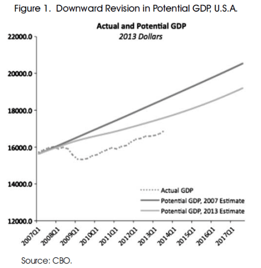
Actual and potential GDP in the USA
26 Jun 2014 Leave a comment
Thinking on the Margin: Principles of Macroeconomics: Every Graph You Need to Know
25 Jun 2014 Leave a comment
What did fiscal policy do in World War II?
23 Jun 2014 Leave a comment
in fiscal policy, macroeconomics Tags: fiscal policy, Lee Ohanian, Robert Barro
It is ironic that both camps use World War II as evidence that the fiscal policy might work (Keynesian macroeconomics) or it does not work (Barro and Ohanian).
The nature of the new spending and how it was financed both matter, as does whether the new spending was a public good, a private good or a general or contingent income transfer matter, and whether the new spending was tax or bond financed all matter to the income and substitution effects of taxes and the additional public debt.
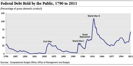
World War II was a temporary increase in government military purchases that will be followed by a long period of primary budget surpluses and perhaps surprise spikes in price inflation to pay down the massive wartime debt.
- A military build-up financed by debt lowers consumer wealth which induces households to consume less leisure and work more while the temporary nature of the fiscal shock increases labour input through inter-temporal substitution of labour into the period of lower taxes.
- The increase in the supply of labour leads to a fall in productivity and real wages. Inter-temporal substitution of labour also raises the real interest rate and lowers private investment.
Barro found that World War II U.S. defence expenditures increased by $540 billion per year at the peak in 1943-44, amounting to 44% of real GDP. this increased real GDP by $430 billion per year in 1943-44 – a multiplier was 0.8 (430/540). The main declines were in private investment, non-military government purchases, and net exports. Wartime production was a dampener, rather than a multiplier.
The war-based multiplier of 0.8 overstates the multiplier that would apply to peacetime government purchases. Public spending crowds out private spending wartime because of intertemporal substitution of labour and consumption smoothing so private investment falls substantially.
People expect the added wartime spending to be temporary so consumer demand will fall by less. Consumers saving less to smooth out the changes in consumption relative the changes in their current after-tax income if the war is expected to last no more than a few years and no major destruction of capital stock and population is anticipated.
Korean War expenditures were financed mostly by higher taxes resulted in a much lower output and welfare compared to the tax smoothing policy for World War II.
The US borrowed heavily to finance World War II as did for most of its previous wars. This means the tax rises necessary to pa for the war debt were spread over a much longer period of time and would in consequence have less effect on labour supply and investment.
In the Korean War, taxes were increased immediately to finance the war. In consequence,labour supply and investment dropped immediately during the period of high taxes
Britain taxed capital income at a much higher rate than the United States during the war and for much of the post-war period. Lee Ohanian explains what happened:
British capital income tax rates rose substantially during the war—they approached 90 per cent—and remained high after it.
Not surprisingly, savings and investment were close to zero over this period, reflecting the very low after-tax return to savings.
In time, London reduced tax rates on savings and investment—and, as a result, savings and investment began to rise, increasing from about 3 per cent of British GDP in the early 1950s to 20 per cent of GDP in the 1980s.
But before its capital income tax rates fell, the United Kingdom was among the slowest growing countries in the industrialized West.
Milton Friedman on the future of the Euro
23 Jun 2014 Leave a comment
in currency unions, Euro crisis, macroeconomics, Milton Friedman Tags: Euro, optimal currency areas
I think the euro is in its honeymoon phase. I hope it succeeds, but I have very low expectations for it.
I think that differences are going to accumulate among the various countries and that non-synchronous shocks are going to affect them. Right now, Ireland is a very different state; it needs a very different monetary policy from that of Spain or Italy.
You know, the various countries in the euro are not a natural currency trading group. They are not a currency area. There is very little mobility of people among the countries.
They have extensive controls and regulations and rules, and so they need some kind of an adjustment mechanism to adjust to asynchronous shocks—and the floating exchange rate gave them one. They have no mechanism now.
If we look back at recent history, they’ve tried in the past to have rigid exchange rates, and each time it has broken down. 1992, 1993, you had the crises. Before that, Europe had the snake, and then it broke down into something else.
So the verdict isn’t in on the euro. It’s only a year old. Give it time to develop its troubles (2000)
AND
The drive for the Euro has been motivated by politics not economics.
The aim has been to link Germany and France so closely as to make a future European war impossible, and to set the stage for a federal United States of Europe.
I believe that adoption of the Euro would have the opposite effect.
It would exacerbate political tensions by converting divergent shocks that could have been readily accommodated by exchange rate changes into divisive political issues.

Taxes and the labour supply in Europe
20 Jun 2014 Leave a comment
in applied price theory, labour economics, labour supply, macroeconomics Tags: labour supply, taxes

Richard Rogerson, 2008. "Structural Transformation and the Deterioration of European Labor Market Outcomes", Journal of Political Economy found that:
1. Hours worked per adult in France, Germany, Italy Europe decline by almost 45% compared to the US since 1956
2. The decline occurs at a steady pace from 1956 until the mid 1990s, in contrast to the fact that the relative increase in unemployment occurs in the mid 1970s.
3. The decline in hours worked in Europe is almost entirely accounted for by the fact that Europe develops a much smaller service sector than the US.
4. Relative increases in taxes and technological catch-up can account for most of the differences between the European and American time allocations to the market and outside over this per.
Ohanian, Rao and Rogerson 2008 in "Work and taxes: allocation of time in OECD countries" found
1. A steep decline in average hours worked per adult and large variations across OECD member countries in the magnitude of this decline.
2. Changes in labour taxes accounted for a large share of the trend differences.
3. Countries with high tax rates devote less time to market work, but more time to home activities, such as cooking and cleaning.
4. This reallocation of time from market work to home work is much stronger for females than for males.
The higher elasticities of labour supply of women, and married women and mothers are beyond dispute. Modern empirical labour economics as led by Mincer was built around explaining female and joint labour supply.
Richard Rogerson, 2007 in "Taxation and market work: is Scandinavia an outlier?" Economic Theory, found that how the government spends tax revenues when assessing the effects of tax rates on aggregate hours of market work.
1. Different forms of government spending imply different elasticities of hours of work with regard to tax rates.
2. While tax rates are highest in Scandinavia, hours worked in Scandinavia are significantly higher than they are in Continental Europe with differences in the form of government spending can potentially account for this pattern.
3. There is a much higher rate of government employment and greater expenditures on child and elderly care in Scandinavia.
Examining how tax revenue is spent is central to understanding labour supply effects:
1. If higher taxes fund disability payments which may only be received when not in work, the effect on hours worked is greater relative to a lump-sum transfer.
2. If higher taxes subsidise day care for individuals who work, then the effect on hours of work will be less than under the lump-sum transfer case.
Crony capitalism flashback – who voted against the TARP in 2008?
20 Jun 2014 Leave a comment
in financial economics, global financial crisis (GFC), great recession, macroeconomics, rentseeking Tags: crony capitalism, TARP
The US House of Representatives initially voted down the TARP in a grand coalition of right-wing republicans and left-wing democrats, voting 205–228. The right-wing republicans opposed the bailout because capitalism is a profit AND loss system. Democrats voted 140–95 in favour of the Bill while Republicans voted 133–65 against it.
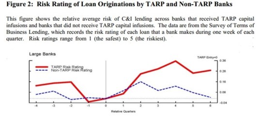
The chart above shows that the degree of risk in commercial loans made by TARP recipients appears to have increased. This is no surprise. In the 1960s, Sam Peltzman published a paper in in the 1960s showing that when deposit insurance was introduced in the USA in the 1930s, the banks halve their capital ratios. They did not need to have as much capital as before to back their lending. The chart below shows that the TARP really didn’t do much for economic policy uncertainty.

In an open letter sent to Congress, over 100 university economists described three fatal pitfalls in the TARP:
1) Its fairness. The plan is a subsidy to investors at taxpayers’ expense. Investors who took risks to earn profits must also bear the losses. The government can ensure a well-functioning financial industry without bailing out particular investors and institutions whose choices proved unwise.
2) Its ambiguity. Neither the mission of the new agency nor its oversight is clear. If taxpayers are to buy illiquid and opaque assets from troubled sellers, the terms, timing and methods of such purchases must be crystal clear ahead of time and carefully monitored afterwards.
3) Its long-term effects. If the plan is enacted, its effects will be with us for a generation. For all their recent troubles, America’s dynamic and innovative private capital markets have brought the nation unparalleled prosperity. Fundamentally weakening those markets in order to calm short-run disruptions is will short-sighted.
A recent IMF study of 42 systemic banking crises showed that in 32 cases, there was government financial intervention.
Of these 32 cases where the government recapitalised the banking system, only seven included a programme of purchase of bad assets/loans (like the one proposed by the US Treasury). These countries were Mexico, Japan, Bolivia, Czech Republic, Jamaica, Malaysia, and Paraguay.
The Government purchase of bad assets was the exception rather than the rule in banking crises and rightly so. The TARP mostly benefited bank shareholders. A case of privatising the gains and socialising the losses from banking was passed on the votes of Congressional Democrats.
A different view of the start of Great Depression | Lee Ohanian
19 Jun 2014 Leave a comment
in great depression, macroeconomics Tags: great depression, Lee Ohanian, Milton Friedman
Friedman and Schwartz argue that the great depression was caused by a collapse of the money supply due to the negligence of the Fed that turned what should have been a garden-variety recession that started in late 1929.
Lee Ohanian argues that there was a steep industrial decline in the USA in 1929 began before monetary contractions or banking panics in 1930 and 1933. The figure below shows manufacturing industry hours worked between January 1929 and September 1930, and measures of the money stock from Friedman and Schwartz corresponding to M1 and M2. Manufacturing industry hours decline substantially and abruptly in late 1929 while money supply fall only about 4% and 1%, respectively.

This sharp decline in the manufacturing sector (a decline of nearly 30% by the fall of 1930 )began before monetary contraction or banking panics – the conventional culprits:
- There are no significant banking panics in 1929 and 1930. The banking panics in the great depression were mostly in 1933 and in 1934.
- Manufacturing hours worked had already fallen by 30% against trend by the time of the first banking panics in 1931, and these first banking panics had minor macroeconomic effects.
The data in the above figure shows that a factor other than monetary contractions or bank runs were central to the onset of the Great Depression.
Nominal wages declined by little during the early stages of the Depression. in September 1931 nominal wage rates were 92 per cent of their level two years earlier. Since a significant price deflation had occurred during these two years, real wages rose by 10 per cent during the same period, while gross domestic product fell by 27 per cent.
With a substantial depression in employment mostly in the manufacturing sector, any explanation of the onset of the great depression in the United States must start with an explanation of why the labour market failed to clear in that sector, why manufacturing decline was so immediately severe before significant monetary contraction and banking panics, why the Depression was so asymmetric across sectors, and provide a theory for why industrial sector wages were persistently well above their market-clearing level.
Just to make it harder for you,nominal wages in the agricultural sector will fell by 40% over the same period in which wages in the manufacturing sector did not fall to all. As Ohanian notes:
The Depression was the first time in the history of the US that wages did not fall during a period of significant deflation.”
Any explanation based on wage rigidity or sluggish wage adjustment or employee resistance to wage cuts must explain why this resistance was so effective in the manufacturing sector but so ineffective in the agricultural sector. Ohanian concluded that:
…the Depression is the consequence of government programs and policies, including those of Hoover, that increased labour’s ability to raise wages above their competitive levels.


Recent Comments